Last week, I posted a discussion in which I stated Bill Russell was a greater “statistical” player compared to Wilt Chamberlain. Expectantly, most replies were in disagreement. The general framework of my opposition would go as follows:

Chamberlain averaged more points, rebounds, and assists per game than Russell on a higher true shooting percentage. Is that not enough? Chamberlain accrued 247.3 Win Shares in his career while Russell managed 163.5. But Russell played fewer seasons, so this may not be a fair comparison. Chamberlain contributed .248 Win Shares every 48 minutes while Russell was worth .193 in the same period. “The Record Book” not only had the advantage in the box score but in advanced statistics; therefore he’s the superior “statistical” player, right?

Ballislife

More often than not, stats are viewed in their rawest forms. This means points per game are frequently used for cross-era comparison despite the fluctuating rates (difficulties) at which different court actions occur and the number of chances a player has to accumulate those actions (pace). When presented with the opportunity to convert per-game stats to modern values, the majority of responses are more dismissive, stating true statistical comparisons across eras are simply unfeasible. For a long time, this was thought to be true. It wasn’t until the work of analytical pioneers that we were given a good idea as to what an “n” points-per-game scorer in 1970 would average fifty years later.

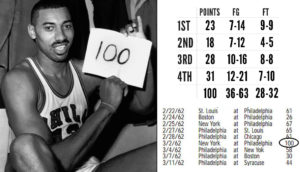
“Inflation-adjusted” statistics emerged to widespread attention just last year, and the results have been extremely promising… and unemployed. The classic example of converting historical values to modern values is Chamberlain’s 50 points-per-game season. It’s mostly recognized that “The Dipper’s” scoring production wouldn’t equate to the same degree in later times, but exactly how much would his 50.4 points per game change? To start, we’d convert points per game to points per-100 (possessions) using Chamberlain’s raw points per game and his team’s number of possessions per game. (Minutes for teams weren’t calculated until the mid-60s, so we’re praying teams didn’t pass too far over the 48 minutes per game threshold). Chamberlain averaged 38.0 points per 100 possessions, which would rank eighth in the league today. He’s often criticized for such, but here we’ll incorporate a key element of adjusting for inflation: it was harder to score a point back then than it is now.

NBA.com

During the 1962 season, offenses scored 93.6 points every 100 possessions, a clear downgrade from 2020’s average offensive rating of 110.6 points. Based on these rates, we can incorporate a factor to weigh ’62 scoring to ’20 scoring. Chamberlain scored 45.4 “inflation-adjusted” points every 100 possessions. If he played in today’s game, “Wilt the Stilt” would average roughly 34.1 points per 75 possessions. Despite his raw scoring rate, Chamberlain’s season was still historical, and he’d likely remain the league’s top volume scorer in any given season using these conversions. The last step is to determine how often he’d be on the court; no star would match Chamberlain’s 48.5 minutes per contest nowadays. The standard protocol in this situation is to compare the average of the top-16 minutes per game in 1962 (40.2) to that of 2020 (35.6). Chamberlain would play approximately 43 minutes per game, from which we can estimate he’d score 40.6 points per game in 2020.

These adjustments, although entirely valid, are met with knee-jerk reactions. People tend to work against these measurements to, instead, remain with a more traditional criterion. It’s likely due to the figures from which people are informed; basketball knowledge is generally passed down from generation to generation, so one’s aggregate views won’t likely stray too far away from its predecessor. A portion of a generation’s population is the one to make the advancements we’re familiar with today: metrics like Win Shares and play-by-play data. Today, our best achievement is Regularized Adjusted Plus/Minus (RAPM), and more specifically, Jeremias Engelmann’s PI RAPM. Resultantly, plus/minus data receive a lot of pushback compared to, say, Win Shares: a metric that’s more easily interpretable (e.g. “Player A” has 7 Win Shares, he contributed 7 wins). But a more foreign concept like Plus/Minus is then met with a higher degree of conflict.

Tableau Public

It’s due to the aforementioned reasons that Wilt Chamberlain is ubiquitously recognized as a superior statistical player to Bill Russell. He checks the boxes of greater raw box scores and a greater score in the most popular and explicit advanced statistic. There are multiple drawbacks to this approach. Earlier, we discussed how statistics are often viewed in their rawest forms, and that still holds true; a very small portion of basketball critics are familiar with statistical adjustments to compare box scores across several decades. But the even larger misconception is the value of the box score. Recently, I plotted the correlation between six samples of three-year luck-adjusted RAPM (from Ryan Davis) and three-year box scores. The offensive component held a moderately-strong r-value; but, expectantly, defense isn’t effectively explained by the box score, making the total box score less indicative of a player’s value than the offensive half alone. Namely, the box score isn’t a strong gauge of a player’s overall value. 

This phenomenon explains why a player like Bill Russell, a defensive superstar with minimal offensive impact, is seen as statistically inferior to a player like Wilt Chamberlain, whose offensive value dominates the box score. Statistics like points, assists, turnovers, and field goals are a few of many that measure a player’s offensive court actions. The intuitive and statistical explanatory power of the offensive box score is greater than that of the defensive box score, and most are aware; even those who use the box score as a primary reference of value know steals, blocks, and defensive rebounds are often poor indicators of defensive impact. However, this means offense receives far more consideration than defense in cases like award recognition and player-ranking lists. Offense is easier to quantify, easier to understand, and it often leaves defense in the dust. The lack of evaluator metrics in the 1960s, let alone the lesser number of counting stats, often means older players are primarily recognized for their offense to a higher degree than current players are. 

NBA.com

Players like Bill Russell are in more strenuous situations in accounting for the methods with which people interpret statistics. It’s less a cause of how point values are designated; say, whether a point scored is truly worth a point to the team. Rather, it’s where the limitations of statistics are drawn. Traditionally, it stops once you start seeing player salaries on their Basketball-Reference page. This means statistical inferencing generally adheres to two categories: simple counting stats and impact metrics. After that, the rest is attributed to the eye test and logical reasoning. This approach severely diminishes the expansive methods of statistical inferencing, an example of which perfectly relates to the ’60s era of basketball: Wilt Chamberlain. He’s widely recognized as one of the greatest scorers of all-time, which he is; but the conclusions drawn from that statement vary. The box-centric approach of statistical interpretation states Chamberlain’s historic scoring makes him one of the most dominant offensive players in league history. However, there’s reason to believe these conclusions may be drawn too fast.

James Harden started to explored trade destinations in the earlier stages of the offseason. His three most-desired suitors were the Philadelphia 76ers, Miami Heat, and Brooklyn Nets, the middle of which drew a trivial amount of noise, but it was an endorsed deal regardless. The prospect of placing the league’s best volume scorer on the most efficient postseason offense may make some sense initially. But consider the qualities that made Miami’s offense great: movement, balanced attacks, and teammate synergies. If Harden were in that lineup, he’d disrupt all of them. He’s the purest “black hole” on offense, in the 99th percentile of average seconds per touch. If any player in the league eats into teammates’ possessions more than the rest, it’s Harden. His high-usage style would take away from the variety of contributors the Heat would employ in the Playoff’s later rounds. With the decreasing frequency of possessions among teammates, the chemistry of those synergies would also decline. The acquisition of Harden would have put a cap on the Heat’s offensive ceiling, yet they were a team in no need of more scoring.

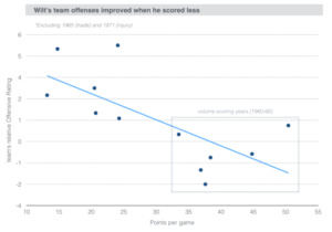
The impact of volume scoring is overstated by the box score, and the great Wilt Chamberlain is no exception. Ben Taylor’s exploratory analysis of Big Musty’s career gave a piece of evidence that was a nail in the coffin for me to make a verdict on the Harden paradigm: there was an extremely-negative correlation between Chamberlain’s shot frequency and his team’s offensive performance. During his thirty-five-to-fifty points-per-game seasons, Chamberlain’s team offenses were often average, wavering above and below that mark at times for only a few points. When he was traded to Philadelphia and his true shooting attempts rapidly declined, their offense took off. There’s no denying the odds of some overstatements due to the unstable roster continuity of Chamberlain’s teams throughout his career, but the general trends hold: high-volume scoring is more of a floor-raising technique than a skill that will truly lift an offense to historical greatness. These concepts are a large part of what makes statistical inferencing so valuable, and the face-value examinations of the box score work against them.

Backpicks

If we apply the same criteria to Russell, determining how certain playstyles relate to team success, we see the opposite: his defensive dominance unlocked historical team defenses. (Due credit to @pdx on Discuss TheGame, who was the one to introduce me to this Russell career trend.) The season before Russ entered the league, the Celtics had the worst-performing defense in basketball. Throw Russell into that lineup, and Boston suddenly becomes the best team defense in a year. The Celtics were an elite defense for every season of Russ’s career, not once allowing opponents to score at a rate more than four points less than league-average; but when he left, their relative defense was raised nearly seven points. Tendencies like these are far greater gauges of a player’s value than a brief overview of the box score because, after all, players only exist to improve team success. They prove a player like Chamberlain may perform well on a team deprived of scoring and in need of posting merely a good team offense, but a player like Russell possesses skills that take a team to dynastical levels. 

How do the 1960s, specifically, prove how we incorrectly interpret statistics? More rigorous statistical methodologies can prove the superior value of a defensive anchor like Bill Russell over a scoring machine like the Big Dipper during an era that was dominated by scoring and without records of defensive counting statistics during good chunks of either players’ career. Despite the lack of full box scores and impact metrics of today, there are still strong measures to gauge the effects of a player’s skills on his team. All it takes is a little more digging.