The introductions of player-evaluation metrics like Player-Impact Plus/Minus (PIPM) and the “Luck-adjusted player estimate using a box prior regularized on-off” (yes, that is actually what “LEBRON” stands for) peddled the use of these metrics to a higher degree than ever. Nowadays, you’ll rarely see a comprehensive player analysis not include at least one type of impact metric. With a growing interest in advanced statistics in the communities with which I am involved, I figured it would serve as a useful topic to provide a more complete (compared with my previous attempts on the subject) and in-depth review of the mathematics and philosophies behind our favorite NBA numbers.

To begin, let’s first start with an all-inclusive definition of what constitutes an impact metric:

“Impact metrics” are all-in-one measurements that estimate a player’s value to his team. Within the context we’ll be diving into here, a player’s impact will be portrayed as his effect on his team’s point differential every 100 possessions he’s on the floor.

As anyone who has ever tried to evaluate a basketball player knows, building a conclusive approach to sum all a player’s contributions in a single notation is nearly impossible, and it is. That’s a key I want to stress with impact metrics:

Impact metrics are merely estimates of a player’s value to his team, not end-all-be-all values, that are subject to the deficiencies and confoundment of the metric’s methodologies and data set.

However, what can be achieved is a “best guess” of sorts. We can use the “most likely” methods that will provide the most promising results. To represent this type of approach, I’ll go through a step-by-step process that is used to calculate one of the more popular impact metrics known today: Regularized Adjusted Plus-Minus, also known as “RAPM.” Like all impact metrics, it estimates the correlation between a player’s presence and his team’s performance, but the ideological and unique properties of its computations make it a building block upon which all other impact metrics rest.

Traditional Plus/Minus

When the NBA started tracking play-by-play data during the 1996-97 season, they calculated a statistic called “Plus/Minus,” which measured a team’s Net Rating (point differential every 100 possessions) while a given player was on the floor. For example, if Billy John played 800 possessions in a season during which his team held a cumulative point differential of 40 points, that player would have a Plus/Minus of +5. The “formula” for Plus/Minus is the point differential of the team while the given player was in the game divided by the number of possessions during which a player was on the floor (a “complete” possession has both an offensive and defensive action), extrapolated to 100 possessions.

Example:

• Billy John played 800 possessions through the season.
• His team outscored its opponents by 40 points throughout those 800 possessions.

Plus/Minus = [(Point Diff / Poss) * 100] = [(40/800) * 100] = +5

While Plus/Minus is a complete and conclusive statistic, it suffers from severe forms of confoundment in a player-evaluation sense: 1) it doesn’t consider the players on the floor alongside the given player. If Zaza Pachulia had spent all his minutes alongside the Warriors mega-quartet during the 2017 season, he would likely have one of the best Plus/Minus scores in the league despite not being one of the best players in the league. The other half of this coin is the players used by the opposing team. If one player had spent all his time against that Warriors “death lineup,” then his Plus/Minus would have been abysmally-low even if he were one of the best players in the game (think of LeBron James with his depleted 2018 Cavaliers).

Adjusted Plus/Minus

“Adjusted” Plus/Minus (APM) was the first step in resolving these issues. The model worked to run through each individual stint (a series of possessions in which the same ten players are on the floor) and distribute the credit for the resulting team performances between the ten players. This process is achieved through the following framework:

(? Squared Statistics)

The system of linear equations is structured so “Y” equals the Net Rating of the home team in stint number “s” in a given game. The variables “A” and “B” are indicators of whether a given player is on the home or away team, respectively, while its first subscript (let’s call it “i”) categorizes a team’s player as a given number and the “s” (the second subscript) numbered stint in which the stint took place.

To structure these equations to divvy the credit of the outcome of the stint, a player for the home team is designated with a 1, a player for the away team is given a -1, and a player on the bench is a 0 (because he played no role in the outcome of the stint).

The matrix form of this system for a full game has the home team’s Net Rating for each stint listed on a column vector, which is then set equal to the “player” matrix, or the 1, -1, and 0 designation system we discussed earlier. Because the matrix will likely be non-square it is non-invertible (another indicator is that the determinant of the matrix would equal zero). Thus, the column vector and the player matrix are both multiplied by the transpose (meaning it is flipped across its diagonal, i.e. the rows become columns and the columns become rows) of the player matrix, which gives us a square matrix to solve for the implied beta column vector!

An example of how a matrix is transposed.

The new column vector will align the altered player matrix with the traditional Plus/Minus of a given player throughout the game while the new player matrix counts the number of interactions between two players. For example, if the value that intersects players one and six has an absolute value of eight, the two of them were on the floor together (or in this case, against each other) for eight stints. Unfortunately, the altered player matrix doesn’t have an inverse either, which requires the new column vector to be multiplied by the generalized inverse of the new player matrix (most commonly used as the Moore-Penrose inverse). I may take a deeper dive into computing the pseudoinverse of a non-invertible matrix in a future walk-through calculation, but the obligatory understanding of the technique for this example is that it’s an approximation of a given matrix with invertible properties.

Multiplying by the “pseudoinverse” results in the approximation of the beta coefficients and will display the raw APM for the players in the game. Taken over the course of the season, a player’s APM is a weighted (by the number of possessions) average of a player’s scores for all games, and voila, Adjusted Plus/Minus! This process serves as the foundation for RAPM and, although a “fair” distribution of a team’s performance, it’s far from perfect. Raw APM is, admittedly, an unbiased measure, but it often suffers from extreme variance. This means the approximations (APM) from the model will often strongly correlate with a team’s performance, but as stated earlier, it’s a “best guess” measurement. Namely, if there were a set of solutions that would appease the least-squares regression even slightly less, the scores could drastically change.

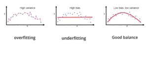
Thanks to the work of statisticians like Jeremias Engelmann (who, in a 2015 NESSIS talk, explained that regular APM will often “overfit,” meaning the model correlates too strongly to the measured response and loses significant predictive power, a main contributor to the variance problem), there are viable solutions to this confoundment.

(? Towards Data Science)

Regularized Adjusted Plus/Minus

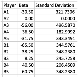
Former Senior Basketball Researcher for the Orlando Magic, Justin Jacobs, in his overview of the metric on Squared Statistics, outlined a set of calculations for APM in a three-on-three setting, obtaining features similar to the ones that would usually be found.

(? Squared Statistics)

Although the beta coefficients were perfectly reasonable estimators of a team’s Net Rating, their variances were astoundingly high. Statistically speaking, the likelihood that a given player’s APM score was truly reflective of his value to his team would be abysmal. To mitigate these hindrances, statisticians use a technique known as a “ridge regression,” which involves adding a very mild perturbation (“change”) to the player interaction matrix as another method to approximate the solutions that would have otherwise been found if the matrix were invertible.

We start with the ordinary least-squares regression (this is the original and most commonly used method to estimate unknown parameters):

This form is then altered as such:

Note: The “beta-hat” indicates the solution is an approximation.

The significant alterations to the OLS form are the additions of the lambda-value and an identity matrix (a square matrix with a “1” across its main diagonal and a “0” everywhere else; think of its usage as multiplying any number by one. Similar to how “n” (a number) * 1 = n, “I” (the identity matrix) * “A” (a matrix) = A). The trademark feature of the ridge regression is its shrinkage properties. The larger the lambda-value grows, the greater the penalty and the APM scores regress closer towards zero.

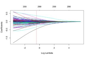
(? UC Business Analytics – an example of shrinkage due to an increase in the lambda-value, represented by its (implied) base-10 logarithm)

With the inclusion of the perturbation to the player interaction matrix, given the properties listed, we have RAPM! However, as with raw APM, there are multiple sources of confoundment. The most damning evidence, as stated earlier, is that we’re already using an approximation method, meaning the “most likely” style from APM isn’t eliminated with ridge regression. If the correlation to team success were slightly harmed, the beta coefficients could still see a change, but not one nearly as drastic as we’d see with regular APM.

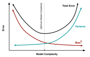
There’s also the minor inclusion of bias that is inherent with ridge regression. The bias-variance tradeoff is another trademark in regression analysis with its relationship between model complexity. Consequently, the goal will often be to find the “optimal” model complexity. RAPM is a model that introduces the aforementioned bias, but it’s such a small inclusion it’s nearly negligible. At the same time, we’re solving the variance problem! It’s also worth noting the lambda-value will affect the beta coefficients, meaning a player’s RAPM is best interpreted relative to the model’s lambda-value (another helpful tidbit from Justin Jacobs).

(? Scott Fortmann-Roe)

My concluding recommendations for interpreting RAPM include: 1) Allow the scores to have time to stabilize. Similar to points per game or win percentage, RAPM varies from game-to-game and, in its earlier stages, will often give a score that isn’t necessarily representative of a player’s value. 2) Low-minute players aren’t always properly measured either. This ties into the sample-size conundrum, but an important aspect of RAPM to consider is that it’s a “rate stat,” meaning it doesn’t account for the volume of a player’s minutes. Lastly, as emphasized throughout the calculation process, RAPM is not the exact correlation between the scoreboard and a player’s presence. Rather, it is an estimate. Given sufficient time to stabilize, it eventually gains a very high amount of descriptive power.

Regression Models

RAPM may be a helpful metric to use in a three or five-year sample, but what if we wanted to accomplish the same task (estimate a player’s impact on his team every 100 possessions he’s on the floor) with a smaller sample size? And how does all this relate to the metrics commonly used today, like Box Plus/Minus, PIPM, and LEBRON? As it turns out, they are the measurements that attempt to answer the question I proposed earlier: they will often replicate the scores (to the best of their abilities) that RAPM would distribute without the need for stabilization. Do they accomplish that? Sometimes. The sole reason for their existence is to approximate value in short stints, but that doesn’t necessarily mean they need some time to gain soundness.

Similar to our exercise with a general impact metric, which uses any method to estimate value, let’s define the parameters of a “regression model” impact metric:

A regression model is a type of impact metric that estimates RAPM over a shorter period of time than needed by RAPM (roughly three years) using a pool of explanatory variables that will vary from metric to metric.

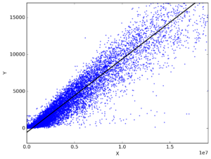
The idea is fairly clear: regression models estimate RAPM (hence, why scores are represented through net impact every 100 possessions). But how do they approximate those values? These types of impact metrics use a statistical technique named the multiple linear regression, which fulfills the goal of the regression model by estimating a “response” variable (in this case, RAPM) using a pool of explanatory variables. This will involve creating a model that takes observed response values (i.e. preexisting long-term RAPM) and its correlation with the independent variables used to describe the players (such as the box score, on-off ratings, etc.).

(? Cross Validated – Stack Exchange)

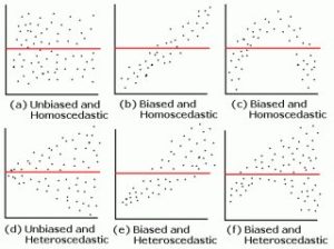
Similar to the “line of best fit” function in Google Sheets that creates forecast models for simple (using one explanatory variable) linear regressions, the multiple linear regression creates a line of best fit that considers descriptive power between multiple explanatory variables. Similar to the least-squares regression for APM, a regression model will usually approximate its response using ordinary least-squares, setting forth the same method present in the RAPM segment that is used to create the perturbation matrix. However, this isn’t always the case. Metrics like PIPM use a weighted linear regression (AKA weighted least squares) in which there is a preexisting knowledge of notable heteroscedasticity in the relationship between the model’s residuals and its predicted values (in rough layman’s terms, there is significant “variance” in the model’s variance).

(The WLS format – describing the use of the residual and the value predicted from the model.)

WLS is a subset of generalized least squares (in which there is a preexisting knowledge of homoscedasticity (there is little to no dispersion among the model’s variance) in the model), but the latter is rarely used to build impact metrics. Most metrics will follow the traditional path of designating two data sets: the training and validation data. The training data is used to fit the model (i.e. what is put into the regression) while the validation data evaluates parts like how biased the model is and assuring the lack of an overfit. If a model were trained to one set of data and not validated by another set, there’d be room to question its status as “good” unless verified at a later date.

After the model is fitted and validated, an impact metric has been successfully created! Unfortunately (again…), we’re not done here, as another necessary part of understanding impact metrics is a working knowledge of how to assess their accuracy.

Evaluating Regression Models

While the formulations of a lot of these impact metrics may resemble one another, that doesn’t automatically mean similar methods produce similar outputs. Intuitively speaking, we’d expect a metric like PIPM or RAPTOR, which includes adjusted on-off ratings and tracking data, to have a higher descriptive power compared to a metric like BPM, which only uses the box score. Most of the time, our sixth sense can pick apart from the good from bad, and sometimes the good and the great, but simply skimming a metric’s leaderboard won’t suffice when evaluating the soundness of its model.

The initial and one of the most common forms of assessing the fit of the model includes the output statistic “r-squared” (R^2), also known as the coefficient of determination. This measures the percent of variance that can be accounted for in a regression model. For example, if a BPM model has an R^2 of 0.70, then roughly 70% of the variance is accounted for while 30% is not. While this figure serves its purpose to measure the magnitude of the models’ fit to its response data, a higher R^2 isn’t necessarily “better” than a lower one. A model that is too reliant on its training data loses some of its predictive power, as stated earlier, falling victim to a model overfit. Thus, there are even more methods to assess the strength of these metrics.

(? InvestingAnswers)

Another common and very simple method could be to compare the absolute values of the residuals of the model’s scoring between the training data and the validation data (we use the absolute values because ordinary least-squares is designed so the sum of the residuals will equal zero) to assess whether the model is equally unbiased toward the data it isn’t fitted to. Although this may be a perfectly sound technique, its simplicity and lack of comprehension may leave the method at a higher risk of error. Its place here is more to provide a more intelligible outlook on evaluating regression models. Similarly, we’ll sometimes see the mean absolute error (MAE) of a model given with the regression details as a measure of how well it predicts those original sets of data.

There’s also the statistical custom of assessing a metric’s residual plot, which compares the model’s predicted value and its residual (observed value minus predicted value) on the x and y-axes, respectively, on a two-dimensional Cartesian coordinate system (AKA a graph). If there is a distinct pattern found within the relationship between the two, the model is one of a poorer fit. The “ideal” models have a randomly distributed plot with values that don’t stray too far from a standardized-zero. Practically speaking, the evaluation of the residual plot is one of the common and viable methods to assessing how well the model was fit to the data.

(? R-bloggers)

However, as seen in works from websites like Nylon Calculus and Dunks & Threes, the most common form of impact metric evaluation in the analytics community is retrodiction testing. This involves using minute-weighted stats from one season used to predict the next season. For example, if Cornelius Featherton was worth +5.6 points every 100 possession he was on the floor during the 2019 season and played an average of 36 minutes per game in the 2020 season, his comparison score would equate to roughly +4.2 points per game. This would be used to measure the errors between a team’s cumulative score (i.e. an “estimated” SRS) against the team’s actual SRS. Evidently, this method suffers from the omission of ever-changing factors like a player’s improvements and declinations, aging curves, and yearly fluctuations, it does hold up against injury and serves a purpose as a measure of predictive power. (“A good stat is a predictive stat” – a spreading adage nowadays.)

Basketball analytics and impact metrics may appear to be an esoteric field at times – I certainly thought so some time ago – but the comprehension of its methodologies and principles isn’t full of completely unintelligible metric designs and reviews. Hopefully, this post served as a good introductory framework to the models and philosophies of the numbers we adore as modern analysts or fans, and that it paints a somewhat clear picture of the meanings behind impact metrics.